Data Files, NumPy & Pandas

Basic (text) file handling, NumPy, pandas, and DateTime. For interactive reading and executing code blocks and find b06-pybum.ipynb or Python (Installation) locally along with JupyterLab.

Watch this section in video format

Watch this section as a video on the @hydroinformatics channel on YouTube.

Load and Write Basic Data Files

Data can be stored in many different (text) file formats such as txt or csv files. Python provides the open(file) and write(...) functions to read and write data from nearby every text file format. In addition, there are packages such as csv (for csv files), which simplify handling specific file types. The following sections illustrate the use of the load(file) and write(...) functions. The later shown pandas module provides more functions to import and export numeric data along with row and column headers.

Load (Open) Text File Data

The open command loads text files as file object in Python. The syntax of the open command is:

open("file-name", "mode")

where:

• file-name is the file to open (e.g., "data.txt"); if the file is not in the script directory, the filename needs to be extended by the full directory (path) to the data file (e.g., "C:/experiment1/data.txt").

• mode defines the access type and it can take the following values:

  • "r" - read-only (default value if no "mode" value is provided); the file cannot be modified nor overwritten.

  • "rb" - read-only in binary format; the binary format is advantageous if the file is not a text file but media such as pictures or videos.

  • "r+" - read and write.

  • "w" - write-only; a new file is created if a file with the provided file-name does not yet exist.

  • "wb" - write-only in binary mode.

  • "w+" - create, write and read.

  • "wb+" - write and read in binary mode.

  • "a" - append new data to a file; the write-pointer is placed at the end of the file and a new file is created if a file with the provided file name does not yet exist.

  • "ab" - append new data in binary mode.

  • "a+" - both append (write at the end) and read.

  • "ab+" - append and read data in binary mode.

When "r" or "w" modes are used, the file pointer (i.e, the blinking cursor that you can see, for example, in Word documents) is placed at the beginning of the file. For "a" modes, the file pointer is placed at the end of the file.

It is good practice to read and write data from and to a file within a with statement to avoid file lock issues. For example, the following code block creates a new text file within a with statement:

with open("data/new.csv", mode="w+") as file:
    file.write("And yet it moves.")

Read-only

Once the file object is created, we can parse the file and copy the file data content to a desired Python data type (e.g., a list, tuple or dictionary). Parsing the data works with for-loops (other loop types will also work) to iterate on lines and line entries. The lines represent strings and data columns can be separated by using the built-in string function line_as_list = str().split("SEPARATOR"), where "SEPARATOR" can be "," (comma), ";" (semicolon), "\t" (tab), or any other sign. After reading all data from a file, use file_object.close() to avoid that the file is locked by Python and cannot be opened by another program.

The following example opens a text file called pure-numbers.txt (download pure-numbers.txt into a local sub-folder called data) that contains float numbers between 0.0 and 10.0. The file has 17 data rows (e.g., for 17 experimental runs) and 4 data columns (e.g., for 4 measurements per experimental run), which are separated by a TAB ("\t" separator) The below code block uses the built-in function readlines() to parse the file lines, splits the lines using the "\t" separator, and loops over the line entries to append them to the list variable data_list only if entry is numeric (verified with the try - except statement). data_list is a nested list that is initiated at the beginning of the script and a sub-list (nested list) is appended for every file line (row).

file_object = open("data/pure-numbers.txt")  # read file with default "mode"="r"

data_list = []  # this will be a nested list with 17 sub-lists (rows) containing 4 entries (columns)=

for line in file_object.readlines():
    line_as_list = line.split("\t")  # converts the line into a list using a tab (\t) separator
    data_list.append([])  # append an empty sub-list for every file line (17 rows)
    for entry in line_as_list:
        try:
            # try to append the entry as floating point number to the last sub-list, which is pointed at using [-1]
            data_list[-1].append(float(entry))
        except ValueError:
            # if entry is not numeric, append 0.0 to the sub-list and print a warning message
            print("Warning: %s is not a number. Replacing value with 0.0." % str(entry))

# verify that data_list contains the 17 rows (sub-lists) with the built-in list function __len__()
print("Number of rows: %d" % data_list.__len__()) 

# verify that the first sub-list has four entries (number of columns)
print("Number of columns: %d" % data_list[0].__len__())

file_object.close()  # close file (otherwise it will be locked as long as Python is still running!) alternative: use with-statement
print(data_list)  # print the data

Number of rows: 17
Number of columns: 4
[[2.59, 5.44, 4.06, 4.87], [4.43, 1.67, 1.26, 2.97], [4.04, 8.07, 2.8, 9.8], [2.25, 5.32, 0.04, 5.57], [6.26, 6.15, 5.98, 8.91], [7.93, 0.85, 5.88, 5.4], [4.72, 1.29, 4.18, 2.46], [7.03, 1.43, 5.53, 9.7], [5.2, 7.87, 1.44, 1.13], [3.18, 5.38, 3.6, 7.32], [5.37, 0.62, 5.29, 4.26], [3.48, 2.26, 3.11, 7.3], [1.36, 1.68, 3.38, 6.4], [1.68, 2.31, 9.29, 3.59], [1.33, 1.73, 3.98, 5.74], [2.38, 9.69, 0.06, 4.16], [9.3, 6.47, 9.14, 3.33]]

Tip

Recall the with statement from the above example. With the with statement, we do not have to write file.close().

Create and Write Files

A file is created with the "w" or "a" modes (e.g., open(file_name, mode="a")).

Tip

When mode="w", the provided file is opened with the pointer at position zero. Writing data will make the pointer overwrite any existing data at the position. That means any existing data in the opened file will be overwritten. To avoid overwriting data in an existing file use mode="a".

Imagine that the above-loaded data_list represents measurements in mm and we know that the precision of the measuring device was 1.0 mm. Thus, all data smaller than 1.0 are within the device error margin, which we want to exclude from further analyses by overwriting such values with nan (not-a-number). For this purpose, we first create a new list variable new_data_list, where we append nan values if data_list[i, j] <= 1.0 and otherwise we preserve the original numeric value of data_list. With open("data/modified-data.csv", mode="w+"), we create a new csv (comma-separated values) file in the data sub-folder. A for-loop iterates on the sub_lists of new_data_list and joins them with a comma-separator. In order to join the list elements of i (i.e., the sub-lists) with ", ".join(list_of_strings)", all list entries first need to be converted to strings, which is achieved through the expression [str(e) for e in row]. The "\n" string needs to be concatenated at the end of every line to create a line break ("\n" itself will not be visible in the file). The command new_file.write(new_line) writes the sub-list-converted-to-string to the file "data/modified-data.csv". Once again, new_file.close() is needed to avoid that the new csv file is locked by Python (alternatively: use a name space within a with statement).

# create a new list and overwrite all values <= 1.0 with nan
new_data_list = []  
for i in data_list:
    new_data_list.append([])
    for j in i:
        if j <= 1.0:
            new_data_list[-1].append("nan")
        else:
            new_data_list[-1].append(j)

print(new_data_list)
# write the modified new_data_list to a new text file
new_file = open("data/modified-data.csv", mode="w+")  # lets just use csv: Python does not care about the file ending (could also be file.wayne)
for row in new_data_list:
    new_line = ", ".join([str(e) for e in row]) + "\n"
    new_file.write(new_line)
new_file.close()

[[2.59, 5.44, 4.06, 4.87], [4.43, 1.67, 1.26, 2.97], [4.04, 8.07, 2.8, 9.8], [2.25, 5.32, 'nan', 5.57], [6.26, 6.15, 5.98, 8.91], [7.93, 'nan', 5.88, 5.4], [4.72, 1.29, 4.18, 2.46], [7.03, 1.43, 5.53, 9.7], [5.2, 7.87, 1.44, 1.13], [3.18, 5.38, 3.6, 7.32], [5.37, 'nan', 5.29, 4.26], [3.48, 2.26, 3.11, 7.3], [1.36, 1.68, 3.38, 6.4], [1.68, 2.31, 9.29, 3.59], [1.33, 1.73, 3.98, 5.74], [2.38, 9.69, 'nan', 4.16], [9.3, 6.47, 9.14, 3.33]]

Modify Existing Files

Existing text files can be opened and modified in either mode="r+" (pretending that information needs to be read before it is modified) or mode="a+". Recall that "r+" will place the pointer at the beginning of the file and "a+" will place the pointer at the end of the file. Thus, if we want to modify lines or entries of an existing file, "r+" is the good choice and if we want to append data at the end of the file, "a" is the good choice (+ is not strictly needed in the case of "a"). This section shows two examples: (1) modification of existing data in a file using "r+", and (2) appending data to an existing file using "a".

Example 1 - Replace data in an existing file with "r+"

In the previous code block, we eliminated all measurements that were smaller than 1 mm because of the precision of the measurement device. However, we have retained all other values with two-digit accuracy - an accuracy that is not given. Consequently, all decimal places in the measurements must also be eliminated. To achieve this, we have to round all measured values with Python’s built-in round function (round(number, n-digits)) to zero decimal places (i.e., n-digits = 0). In this example (featured in the below code block), an exception IOError is raised when the file "data/modified-data.csv" does not exist (or if it is locked by another software). An if statement ensures that rounding the data is only attempted if the file exists. The overwriting procedure first reads all lines of the file into the lines variable. After reading all lines, the pointer is at the end of the file, and file.seek(0) puts the pointer back to position 0 (i.e., at the beginning of the file). file.truncate() purges the file. Thus, the original file is blank for a moment and all file contents are stored in the lines variable. Rounding the data happens within a for-loop that:

• Splits the comma-separated line string (produces lines_as_list).

• Creates the temporary list _numeric_line_, where rounded, numeric values are stored (the variable is overwritten in every iteration).

• Loops over the line entries (line_as_list), where an exception statement appends rounded (to zero digits), numeric values and appends "nan" when an entry is not numeric.

• Writes the modified line to the "data/modified-data.csv" csv file.

Finally, the csv is closed with modified_file.close().

try:
    modified_file = open("data/modified-data.csv", mode="r+")  # re-open the above data file in read-write
except IOError:
    print("The file does not exist.")
    
if modified_file:
    # go here only if the file exists
    lines = modified_file.readlines()  # read lines > pointer moves to file end
    modified_file.seek(0)  # return pointer to file beginning
    modified_file.truncate()  # clear file content
    for line in lines:
        line_as_list = line.split(", ")  # converts the line into a list using comma separator
        _numeric_line_ = []
        for e in line_as_list:
            try: 
                _numeric_line_.append(round(float(e), 0))  # try to convert line entry to float and round to 0 digits
            except ValueError:
                _numeric_line_.append(e)  # for nan values 
        # write rounded values
        modified_file.write(", ".join([str(e) for e in _numeric_line_]) + "\n")
    print("Processed file." )
    modified_file.close()
    

Processed file.

Theoretically the above code snippet can be re-written as a function to modify any data in a file. In addition, other threshold values or particular data ranges can be filtered using if - else statements.

Example 2 - Append data to an existing file with "a+"

By coincidence, you find a hand-written measurement protocol that has data of an 18th experimental run, which is not in the electronic measurement data file due to a data transmission error. Now, you want to add the data to the above-produced csv file. Entering the data does not take much work, because only 4 measurements were performed per experimental run and the below code block contains the hand-written data in a list variable called forgotten_data. This example uses the os module (recall Packages, Modules and Libraries) to verify if the data file exists with os.path.isfile() (the os.getcwd() statement is a gadget here). The code block features the usage of a with statement (i.e., a with - context manager or name space).

The essential part of the code that writes the line to the data file is file.write(line), where line corresponds to the above-introduced ", ".join(list-of-strings) + "\n" string.

import os
print(os.getcwd())
forgotten_data = [4.0, 3.0, "nan", 8.0]

if os.path.isfile("data/modified-data.csv"):
    with open("data/modified-data.csv", mode="a") as file_object:
        file_object.write(", ".join([str(e) for e in forgotten_data]) + "\n")
    print("Data appended.")
else:
    print("The file does not exist.")

Challenge

The expression ", ".join([str(e) for e in a_list]) + '\n' is a recurring expression in many of the above-shown code blocks. How does a function look like that automatically generates this expression for lists of different data types?

NumPy

NumPy provides high-level mathematical functions for linear algebra including operations on multi-dimensional arrays and matrices. The open-source NumPy (for Numerical Python) library is written in Python and C, and comes with comprehensive documentation (download the latest version on the developer’s web site or read the developer’s online tutorial).

Watch the NumPy section in video format

Watch this section as a video on the @hydroinformatics channel on YouTube.

Installation

NumPy can be installed through Anaconda (recall instructions) and the developers recommend using a scientific Python distribution (Anaconda) with SciPy Stack.

The provided Anaconda environment.yml (flussenv) already includes NumPy (more information in the installation section). Similarly, Linux users will have NumPy installed in a virtual environment (e.g., vflussenv) with pip (recall pip-installing flusstools). Otherwise, to install NumPy in any other conda environment, open Anaconda Prompt (Start > type Anaconda Prompt) and type:

conda activate ENVIRONMENT-NAME
conda install numpy

To pip-install NumPy in any other virtual environment tap:

pip install numpy

Usage

The NumPy library is typically imported with import numpy as np. Array handling is the foundation of NumPy and linear algebra, where arrays represent a kind of nested data lists. To create a NumPy array, use np.array((values)), where values is a sequences of values.

Tip

This section provides insights into basic NumPy functions and it does not (rather: cannot) cover all NumPy functions and data types. Generally speaking, be sure that whatever mathematical operation you want to perform, NumPy offers a solution. Check out the NumPy documentation, have a look at NumPy’s built-in functions and methods overview, or use your favorite search engine with the search words numpy FUNCTION.

The following code block shows very basic usage of NumPy (or: numpy) imported as np and the creation of a 2x3 numpy array. The rounded parentheses indicated that the value sequence of the np.array represents a tuple for creating a multi-dimensional array.

import numpy as np
an_array = np.array(([2, 3, 1], [4, 5, 6]))
print(an_array)

[[2 3 1]
 [4 5 6]]

NumPy arrays (data type: ndarray) have many built-in features, for example to output the array size:

print(type(an_array))
print("Array dimensions: " + str(an_array.shape))
print("Total number of array elements: " + str(an_array.size))
print("Number of array axes: " + str(an_array.ndim))

<class 'numpy.ndarray'>
Array dimensions: (2, 3)
Total number of array elements: 6
Number of array axes: 2

There are many types of np.arrays and many ways to create them:

print(np.array([(2, 3, 1), (4, 5, 6)]))  # the same as an_array
print(np.array([[2, 3, 1], [4, 5, 6]], dtype=complex))

[[2 3 1]
 [4 5 6]]
[[2.+0.j 3.+0.j 1.+0.j]
 [4.+0.j 5.+0.j 6.+0.j]]

Arrays of zeros or ones or empty arrays can be created with integer or float data types. When creating such arrays, be aware of using tuples (i.e., sequences embraced with rounded parentheses) to define array dimensions:

print(np.zeros((2,6)))
print(np.ones((2,6), dtype=np.float64))  # other dtypes: int16, np.int16, float, np.float32, np.complex32
print(np.empty((2,6)))
print(np.empty((2,6), dtype=np.int16))

[[0. 0. 0. 0. 0. 0.]
 [0. 0. 0. 0. 0. 0.]]
[[1. 1. 1. 1. 1. 1.]
 [1. 1. 1. 1. 1. 1.]]
[[1. 1. 1. 1. 1. 1.]
 [1. 1. 1. 1. 1. 1.]]
[[2 0 3 0 1 0]
 [4 0 5 0 6 0]]

Data type sizes

NumPy data types have different sizes (in bytes) and the more digits, the larger the variable size. For example, np.float64 has an item size of 8 bytes (64/8), while np.float32 has an item size of 4 bytes (32/8) only. Use ndarray.itemsize (e.g., an_array.itemsize) to find out the size of an array in bytes. For analyses of large datasets, the data type gets very important regarding computation speed and storage.

NumPy provides the arange(start, end, step-size) function to create numeric sequences. Such sequences represent arrays (ndarray) that can later be reshaped (i.e., re-organized in columns and rows).

print("1D array:")
print(np.arange(0, 10, 2))  # 1D array
print("\n2D array:")
print(np.arange(0, 12, 2).reshape(2, 3))  # 2D array
print("\n3D array:")
print(np.arange(1, 13, 1).reshape(2, 2, 3))  # 3D array
print("\n1D Linspace (start, end, number-of-elements):")
print(np.linspace(0, np.pi, 3))

1D array:
[0 2 4 6 8]

2D array:
[[ 0  2  4]
 [ 6  8 10]]

3D array:
[[[ 1  2  3]
  [ 4  5  6]]

 [[ 7  8  9]
  [10 11 12]]]

1D Linspace (start, end, number-of-elements):
[0.         1.57079633 3.14159265]

Random numbers can be generated with NumPy’s random number generator np.random and its .random(range_tuple) function.

rand_array = np.random.random((2,4))
print(rand_array)

[[0.0204844  0.91185321 0.00152947 0.79774412]
 [0.45685876 0.65600015 0.55038482 0.03690686]]

Built-in array functions enable finding minimum or maximum values, or sums of arrays:

print("Sum of 12-elements ones-array: " + str(np.ones((2,6)).sum()))
print("Minimum: " + str(an_array.min()))
print("Maximum: " + str(an_array.max()))

Sum of 12-elements ones-array: 12.0
Minimum: 1
Maximum: 6

Color Arrays

Arrays may also contain color information, where colors represent a mix of the three base colors red, green, and blue (RGB). Thus, one color can be defined as [red-value, green-value, blue-value], and a value of 0 means that a color tone is not present, while 255 is its maximum value. There is no color when all color tone values are zero, which corresponds to black; when all color tones are maximum (255), the color mix corresponds to white. This way, array elements can be lists of color tones, and plotting such arrays produces images. The following example produces an array with 5 color-list elements, which could be plotted as a very basic image with 5 pixels (one black, red, green, blue, and white, respectively):

color_set = np.array([[0, 0, 0],         # black
                      [255, 0, 0],       # red
                      [0, 255, 0],       # green
                      [0, 0, 255],       # blue
                      [255, 255, 255]])  # white

Array (Matrix) Operations

Array calculations (matrix operations) follow the rules of linear algebra:

A = np.random.random((2,4))
B = np.random.random((4,2))
print("Subtraction: " + str(A.transpose() - B))
print("Element-wise product: " + str(A.transpose() * B))
print("Matrix product (option 1): " + str(A @ B))
print("Matrix product (option 2): " + str(A.dot(B)))

Subtraction: [[ 0.1115262  -0.48000352]
 [ 0.1494478   0.31398052]
 [ 0.38778125  0.18341211]
 [ 0.0014262   0.5411479 ]]
Element-wise product: [[0.78023517 0.24540468]
 [0.01212987 0.11177306]
 [0.04761943 0.21543691]
 [0.37867353 0.05979503]]
Matrix product (option 1): [[1.218658   1.0311045 ]
 [0.73402296 0.63240968]]
Matrix product (option 2): [[1.218658   1.0311045 ]
 [0.73402296 0.63240968]]

Further element-wise calculations include exponential (**), geometric (np.sin, np.cos, np.tan, etc.), and boolean operators:

print("A to the power of 3: " + str(A**3))
print("Exponential: " + str(np.exp(A)))
print("Square root: " + str(np.sqrt(A)))
print("Sine of A times 3: " + str(np.sin(A) * 3))
print("Boolean where A is smaller than 0.3: " + str(A < 0.3))

A to the power of 3: [[0.83278802 0.00897507 0.11465192 0.23383377]
 [0.02992313 0.14581371 0.18020002 0.25637808]]
Exponential: [[2.56210893 1.23098678 1.62548021 1.85165172]
 [1.36404919 1.69272506 1.7591499  1.88753709]]
Square root: [[0.96996429 0.45586852 0.6969959  0.7849064 ]
 [0.55718724 0.72549272 0.75155218 0.79704006]]
Sine of A times 3: [[2.42414331 0.61897047 1.40075657 1.73351616]
 [0.91648323 1.50711546 1.60581841 1.78019148]]
Boolean where A is smaller than 0.3: [[False  True False False]
 [False False False False]]

Array Shape Manipulation

Sometimes it is necessary to stack a multi-dimensional array into a vector or recast the shape of an array. Beyond the reshape() function, there are a couple of other options to manipulate the shape of an array:

print("Flattened matrix A (into a vector):\n" + str(A.ravel()))
print("\nTranspose matrix A and append B:\n" + str(np.array([A.transpose(), B])))
print("\nTranspose matrix A and append B and cast into a (4x4) array:\n" + str(np.array([A.transpose(), B]).reshape(4,4)))

Flattened matrix A (into a vector):
[0.94083072 0.20781611 0.48580329 0.61607806 0.31045762 0.52633969
 0.56483068 0.63527285]

Transpose matrix A and append B:
[[[0.94083072 0.31045762]
  [0.20781611 0.52633969]
  [0.48580329 0.56483068]
  [0.61607806 0.63527285]]

 [[0.82930452 0.79046114]
  [0.05836831 0.21235917]
  [0.09802204 0.38141858]
  [0.61465186 0.09412495]]]

Transpose matrix A and append B and cast into a (4x4) array:
[[0.94083072 0.31045762 0.20781611 0.52633969]
 [0.48580329 0.56483068 0.61607806 0.63527285]
 [0.82930452 0.79046114 0.05836831 0.21235917]
 [0.09802204 0.38141858 0.61465186 0.09412495]]

NumPy File Handling and np.nan

In the above examples on file handling, measurement data were loaded from text files, manipulated (modified), and (re-)written. The data manipulation involved the introduction of "nan" (not-a-number) values, which were excluded because measurements <1 mm were considered errors. Why didn’t we use zeros here? Zeros are numbers, too, and have a significant effect on data statistics (e.g., for calculating mean values). However, the "nan" string value may cause difficulties in data handling, in particular regarding the consistency of function output. NumPy provides with the np.nan data type a powerful alternative to the tedious "nan" string.

NumPy also has a text file load function called np.loadtxt(file-name, *args, **kwargs), which imports text files as np.arrays of float values. The default float value type can be adapted with the optional keyword dtype. Other optional keyword arguments are:

• delimiter=STR (e.g., delimiter=';'), where the default is "None"

• usecols=TUPLE (e.g., usecols=(1, 3) extracts the 2^nd and 4^th column), where also one integer value is possible to read just on single column

• skiprows=INT (e.g., skiprows=2 skips the first two lines), where the default is 0

• more arguments are available and listed in the NumPy documentation.

The following example loads the above-created csv file data/modified-data.csv containing integer and "nan" string values, which are automatically converted to np.nan.

experiment_data = np.loadtxt("data/modified-data.csv", delimiter=",")
print("This is the data 4th line (row): " + str(experiment_data[3, :]))
print("The data type of the 3rd (%s) entry is: " % str(experiment_data[3, 2]) + str(type(experiment_data[3, 2])))

This is the data 4th line (row): [ 2.  5. nan  6.]
The data type of the 3rd (nan) entry is: <class 'numpy.float64'>

In addition, or as an alternative, the function np.load() picks up data from file-like .npz, .npy, or pickled (saved Python objects) data sources (more information is available in the NumPy docs).

Statistics

The above examples featured array functions to assess basic array statistics such as the minimum and maximum. NumPy provides many more functions for array statistics such as the mean, median, or standard deviation, including functions that account for np.nan values. The following example illustrates some of the statistical functions with the experimental data from the above examples. Note the usage of nanmean instead of mean and statistics along array axis, where the optional keyword argument axis=0 corresponds to columns and axis=1 to statistics along rows in 2-dimensional arrays (maximum axis number corresponds to the array dimensions n minus 1, i.e., maximum axis=n-1).

print("Mean value (without nan): " + str(np.mean(experiment_data)))  # no applicable result
print("Mean value with np.nan: " + str(np.nanmean(experiment_data))) 
print("Mean value along axis 0 (columns): " + str(np.nanmean(experiment_data, axis=0))) 
print("Mean value along axis 1 (rows): " + str(np.nanmean(experiment_data, axis=1))) 

Mean value (without nan): nan
Mean value with np.nan: 4.626865671641791
Mean value along axis 0 (columns): [4.11111111 4.25       4.53333333 5.55555556]
Mean value along axis 1 (rows): [4.25       2.5        6.25       4.33333333 6.75       6.33333333
 3.         6.         3.75       4.75       4.66666667 3.75
 3.         4.25       3.25       5.33333333 6.75       5.        ]

The following paragraphs represent a tabular overview of statistical functions in NumPy (source: NumPy v.1.13 docs). The listed functions only represent the baseline and NumPy provides many more options, which can be leveraged using any search engine with NumPy and the desired function as a search keyword.

---

Basic statistic functions

Function	Description
nanmin(a[, axis, out, keepdims])	Minimum of an array or along an axis, ignoring np.nan.
nanmax(a[, axis, out, keepdims])	Maximum of an array or along an axis, ignoring np.nan.
ptp(a[, axis, out])	Range of values (max - min) along an axis.
percentile(a, q[, axis, out, ...])	q-th percentile of data along a specified axis.
nanpercentile(a, q[, axis, out, ...])	q-th percentile of data along a specified axis, ignoring np.nan.

---

Mean (average), standard deviation, and variances

Function	Description
median(a[, axis, out, overwrite_input, keepdims])	Median along an (optional) axis.
average(a[, axis, weights, returned])	Weighted average along an (optional) axis.
mean(a[, axis, dtype, out, keepdims])	Arithmetic mean along an (optional) axis.
std(a[, axis, dtype, out, ddof, keepdims])	Standard deviation along an (optional) axis.
var(a[, axis, dtype, out, ddof, keepdims])	Variance along an (optional) axis.
nanmedian(a[, axis, out, overwrite_input, ...])	Median along an (optional) axis, ignoring np.nan.
nanmean(a[, axis, dtype, out, keepdims])	Arithmetic mean along an (optional) axis, ignoring np.nan.
nanstd(a[, axis, dtype, out, ddof, keepdims])	Standard deviation along an (optional) axis, while ignoring np.nan.

---

Correlating data (arrays)

Function	Description
corrcoef(x[, y, rowvar, bias, ddof])	Pearson (product-moment) correlation coefficients.
correlate(a, v[, mode])	Cross-correlation of two 1-dimensional sequences.
cov(m[, y, rowvar, bias, ddof, fweights, ...])	Estimate covariance matrix, based on data and weights.

---

Generate and plot histograms

Function	Description
histogram(a[, bins, range, normed, weights, ...])	Histogram of a set of data.
histogram2d(x, y[, bins, range, normed, weights])	Bi-dimensional histogram of two data samples.
histogramdd(sample[, bins, range, normed, ...])	Multidimensional histogram of some data.
bincount(x[, weights, minlength])	Count number of occurrences of each value in array of non-negative ints.
digitize(x, bins[, right])	Indices of the bins to which each value in input array belongs.

Can NumPy do MATLAB®?

Are you considering switching to Python after starting softly into programming with MATLAB®-like software? There are many reasons for enhancing data analyses with Python and here are some facilitators for previous MATLAB® users:

• MATLAB® matrices can be loaded and saved with scipy.io.loadmat(matrix-file-name) (use import scipy).

• NumPy’s np.array replaces MATLAB®’s matrix notation (even though there is the historic, deprecated NumPy data type np.matrix).

• Import many MATLAB® features from np.matlib (e.g., from numpy.matlib import rand, zeros, ones, empty, eye) or more generally import numpy.matlib as M).

• Find the NumPy equivalent of many MATLAB® function in the NumPy documentation.

• To emulate MATLAB®’s plot functions use the pylab package and import it as from pylab import *.
  ⚠ This overwrites all other (standard) definitions of the plot() function and array() objects. So this usage is deprecated. Read the plotting section for comprehensive plotting instructions with Python.

MATLAB® is a registered trademark of The MathWorks.

Exercise

Practice numpy and csv file handling in the reservoir design exercise.

Pandas

pandas is a powerful library for data analyses and manipulation with Python. It can handle NumPy arrays, and both packages jointly represent a powerful data processing engine. The power of pandas lies in processing data frames, data labeling (e.g., workbook-like column names), and flexible file handling functions (e.g., the built-in read_csv(csv-file) function). While NumPy arrays enable calculations with multidimensional arrays (beyond 2-dimensional tables) and low memory consumption, pandas DataFrames efficiently process and label tabular data with more than ~100,000 rows. Because of its labelling capacity, pandas also finds broad application in machine learning. In summary, pandas’ functionality builds on top of NumPy and both libraries are maintained by the SciPy (Scientific computing tools for Python) community that also produces matplotlib (see the plotting section) and IPython (Jupyter’s Python kernel).

Watch the pandas section on YouTube

Watch this section as a video on the @hydroinformatics channel on YouTube.

Installation

pandas can be installed through Anaconda (recall instructions) and the developers recommend using a scientific Python distribution (Anaconda) with SciPy Stack.

The provided Anaconda environment.yml (flussenv) already includes pandas (more information in the installation section). Similarly, Linux users will have pandas installed in a virtual environment (e.g., vflussenv) with pip (recall pip-installing flusstools). Otherwise, to install pandas in any other conda environment, open Anaconda Prompt (Start > type Anaconda Prompt) and type:

conda activate ENVIRONMENT-NAME
conda install pandas

To pip-install pandas in any other virtual environment tap:

pip install pandas

Usage

pandas standard import alias is pd: import pandas as pd. The following sections provide an overview of basic pandas functions and many more features are documented in the developer’s docs.

Data Frames & Series

The below code block illustrates one way to create a pandas data frame (pd.DataFrame), one of pandas core objects. Note the difference between a 1-dimensional series pd.Series (corresponds to a one-column data frame), and an n-dimensional data frame with row (=index) and column names. The default row names number rows starting from 0 (unlike Office software that starts at row no. 1), without column names. Column names can be initially defined as a list and replaced with a dictionary that maps the initial list entries to new names.

import pandas as pd

print("A 1-column pd.DataFrame:\n"+ str(pd.Series([3, 4, np.nan])))  # a simple pandas data frame with one column

row_names = np.arange(1, 4, 1)
wb_like_df = pd.DataFrame(np.random.randn(row_names.__len__(), 3), 
                          index=row_names, columns=['A', 'B', 'C'])
print("\nThis is a workbook-like (row and column names) data frame:\n" + str(wb_like_df))
print("\nRename column names with dictionary:\n" + str(wb_like_df.rename(
        columns={'A': 'Series 1', 'B': 'Series 2', 'C': 'Series 3'})))
print("\nTranspose the data frame:\n" + str(wb_like_df.T))

A 1-column pd.DataFrame:
0    3.0
1    4.0
2    NaN
dtype: float64

This is a workbook-like (row and column names) data frame:
          A         B         C
1  1.551689 -0.425844 -1.120399
2 -0.472708 -0.619897 -1.491136
3  1.909126  0.273118 -2.425986

Rename column names with dictionary:
   Series 1  Series 2  Series 3
1  1.551689 -0.425844 -1.120399
2 -0.472708 -0.619897 -1.491136
3  1.909126  0.273118 -2.425986

Transpose the data frame:
          1         2         3
A  1.551689 -0.472708  1.909126
B -0.425844 -0.619897  0.273118
C -1.120399 -1.491136 -2.425986

A pandas DataFrame object can also be created from a dictionary, where the dictionary keys define column names and the dictionary values constitute the data of every column:

df = pd.DataFrame({'Flow depth': pd.Series(np.random.uniform(low=0.1, high=0.3, size=(4,)), dtype='float32'),
                   'Sediment': ["yes", "no", "yes", "no"],
                   'Flow regime': pd.Categorical(["fluvial", "fluvial", "supercritical", "critical"]),
                   'Water': "Always there"})
print("A dictionary-built data frame:\n" + str(df))
print("\nFrame data types:\n" + str(df.dtypes))

A dictionary-built data frame:
   Flow depth Sediment    Flow regime         Water
0    0.210366      yes        fluvial  Always there
1    0.234890       no        fluvial  Always there
2    0.247299      yes  supercritical  Always there
3    0.164717       no       critical  Always there

Frame data types:
Flow depth      float32
Sediment         object
Flow regime    category
Water            object
dtype: object

Built-in attributes and methods of a pandas DataFrame enable easy access to the top (head) and the bottom of a data frame and many more object characteristics (recall: use dir(dict_df) or read the developer’s docs):

print("Head of the dictionary-based dataframe (first two rows):\n" + str(df.head(2)))
print("\nEnd (tail) of the dictionary-based dataframe (last row):\n" + str(df.tail(1)))

Head of the dictionary-based dataframe (first two rows):
   Flow depth Sediment Flow regime         Water
0    0.210366      yes     fluvial  Always there
1    0.234890       no     fluvial  Always there

End (tail) of the dictionary-based dataframe (last row):
   Flow depth Sediment Flow regime         Water
3    0.164717       no    critical  Always there

Example: Create a pandas.DataFrame of Froude Numbers

In hydraulics, the Froude number \(Fr\) characterizes the flow regime as “fluvial” (Fr<1), “critical” (Fr=1), or “super-critical” (Fr>1). The precision of measurement devices in physical flume experiments makes the exact determination of the critical moment a challenge and forces researchers to apply an interval around 1, rather than the exact value of 1.0:

Fr	(0.00, 0.95(	(0.95, 1.00(	(1.00)	)1.00, 1.05)	)1.05, inf(
Flow	fluvial	nearby critical (slow)	critical	nearby critical (fast)	super-critical

pd.DataFrame( ... ) objects are a convenient for to classify and store flume experiment data:

Fr_dict = {0.925: "fluvial", 0.975: "nearby critical (slow)", 1.0: "critical", 1.025: "nearby critical (fast)", 1.075: "super-critical"}
Fr_measured = np.random.uniform(low=0.01, high=2.00, size=(10,))
Fr_classified = [Fr_dict[min(Fr_dict.keys(), key=lambda x:abs(x-m))] for m in Fr_measured]
obs_df = pd.DataFrame({"measured": Fr_measured, "flow regime": Fr_classified})
print(obs_df)

   measured             flow regime
0  1.462930          super-critical
1  0.430861                 fluvial
2  0.998070                critical
3  0.131475                 fluvial
4  0.174419                 fluvial
5  0.455032                 fluvial
6  1.235265          super-critical
7  0.519341                 fluvial
8  0.659579                 fluvial
9  0.978529  nearby critical (slow)

Append Data to a pandas.DataFrame

The at, loc, concat, and append methods of pandas provide direct options for inserting rows or columns into a pd.DataFrame. However, these built-in methods are approximately one order of magnitude slower than taking the detour via a dictionary. This applies especially to data frames with more than 10,000 elements. This means that the fastest method to insert data into a pd.DataFrame is:

1. Convert an existing pd.DataFrame object to a dictionary with pd.DataFrame.to_dict() (e.g., dict_of_df = df.to_dict()).

2. Update the dictionary with the new data

• Append rows with dict_of_df.update{"existing-column-name": {"new-row-name": NEW_DATA}}

• Append columns with dict_of_df.update{"newcolumn-name": {"existing-row-names": NEW_DATA(size=existing-number-of-rows}}

1. Re-convert the dictionary to a pd.DataFrame with df = pd.DataFrame.from_dict(dict_of_df)

The following code block illustrates both adding a row and a column to an existing pandas data frame.

import random

# convert data frame to dictionary
dict_of_obs_df = obs_df.to_dict()

# append new row
new_row_index = max(dict_of_obs_df["measured"]) + 1
dict_of_obs_df["measured"].update({new_row_index: 0.996})
dict_of_obs_df["flow regime"].update({new_row_index: "nearby critical (slow)"})

# append column
dict_of_obs_df.update({"with sediment": {}})
for k in dict_of_obs_df["measured"].keys():
    dict_of_obs_df["with sediment"].update({k: bool(random.getrandbits(1))})

# re-build data frame
obs_df = pd.DataFrame.from_dict(dict_of_obs_df)
print(obs_df.tail(3))

    measured             flow regime  with sediment
8   0.659579                 fluvial          False
9   0.978529  nearby critical (slow)           True
10  0.996000  nearby critical (slow)           True

NumPy Arrays and pandas Data Frames

One major difference between a NumPy array and a pandas DataFrame is that NumPy arrays can only have one single data type (dtype), while a pandas DataFrame can have different data types (one dtype per column). This is why a NumPy array can be seamlessly converted to a pandas DataFrame, but the opposite conversion can cause high computational cost: pandas comes with a built-in function to convert a pandas DataFrame into a NumPy array, where numeric variables are maintained where possible. If one column of the pandas DataFrame is non-numeric, the conversion involves copying the object, which then causes high computational costs. Note that the index and column labels of a pandas DataFrame are lost in the conversion from pd.DataFrame to np.ndarray.

print(obs_df.to_numpy())

[[1.4629304199712003 'super-critical' True]
 [0.4308609175144578 'fluvial' True]
 [0.9980702542754516 'critical' False]
 [0.13147505751224464 'fluvial' False]
 [0.1744193402007127 'fluvial' False]
 [0.45503162541640574 'fluvial' True]
 [1.2352651606844145 'super-critical' True]
 [0.5193413669752244 'fluvial' False]
 [0.6595793984115736 'fluvial' False]
 [0.9785285127361709 'nearby critical (slow)' True]
 [0.996 'nearby critical (slow)' True]]

Access Data Frames Entries

Elements of data frames are accessible by the column and row label (df.loc[index=row, column-label]) or number (df.iloc):

print("Label localization results in: " + str(df.loc[2, "Flow depth"]))
print("Same result with integer grid location: " + str(df.iloc[2, 0]))

Label localization results in: 0.2472994
Same result with integer grid location: 0.2472994

Reshape Data Frames

Single or multiple rows (indices) and columns can be extracted from and combined into new or existing DataFrame objects:

print(pd.DataFrame([df["Flow depth"], df["Sediment"]]))

                   0        1         2         3
Flow depth  0.210366  0.23489  0.247299  0.164717
Sediment         yes       no       yes        no

The df.stack() method pivots the columns of a data frame, which is a powerful tool to classify data that can take different dimensions (e.g., the volume and weight of 1 m³ water - read more about the stack method).

print(df.stack()[0])
df.unstack()  # unstack data frame

Flow depth         0.210366
Sediment                yes
Flow regime         fluvial
Water          Always there
dtype: object

Flow depth   0         0.210366
             1          0.23489
             2         0.247299
             3         0.164717
Sediment     0              yes
             1               no
             2              yes
             3               no
Flow regime  0          fluvial
             1          fluvial
             2    supercritical
             3         critical
Water        0     Always there
             1     Always there
             2     Always there
             3     Always there
dtype: object

Big datasets often contain large amounts of data with many labels, but we are often only interested in a small subset of the data. To this end, data frame subsets can be created with df.pivot(index, columns, **values) (Pivot method):

print("Pivot table for \'Flow regime\':\n" + str(df.pivot(index="Sediment", columns="Flow depth")["Flow regime"]))
print("\nPivot table for \'Water\':\n" + str(df.pivot(index="Sediment", columns="Flow depth")["Water"]))

Pivot table for 'Flow regime':
Flow depth  0.164717 0.210366 0.234890       0.247299
Sediment                                             
no          critical      NaN  fluvial            NaN
yes              NaN  fluvial      NaN  supercritical

Pivot table for 'Water':
Flow depth      0.164717      0.210366      0.234890      0.247299
Sediment                                                          
no          Always there           NaN  Always there           NaN
yes                  NaN  Always there           NaN  Always there

In addition, df.pivot_table(index, columns, values, aggfunc) (Pivot table function) enables inline Office-like function application to one or more rows and/or columns.

print("\'mean\' for \'Flow depth\':\n" + str(df.pivot_table(index="Sediment", columns="Flow regime", values="Flow depth", aggfunc=np.mean)))

'mean' for 'Flow depth':
Flow regime  critical   fluvial  supercritical
Sediment                                      
no           0.164717  0.234890            NaN
yes               NaN  0.210366       0.247299

Read more about reshaping and pivoting data frames in the developer’s docs.

File Handling (csv, Workbooks, and More)

pandas can read from and write to many data file types, which makes it extremely powerful for analyzing any data. The following table summarizes the most important file types for numerical hydraulic, morphodynamic, and fluvial landscape analyses, and more file type handlers can be found at the developer’s docs.

File type	pandas read	pandas write	Usage example
CSV	read_csv	to_csv	Reading from data loggers (e.g., discharge, flow depth)
Google BigQuery	read_gbq	to_gbq	Analyze social media
JSON	read_json	to_json	Manipulate BASEMENT model files
HTML	read_html	to_html	Process web site data
HDF5 Format	read_hdf	to_hdf	Analyze BASEMENT or HEC-RAS output files
Python Pickle Format	read_pickle	to_pickle	Cache memory dump
SQL	read_sql	to_sql	Retrieve and write data to SQL data bases
Workbooks (Excel / Open doc)	read_excel	to_excel	Interface with non-programmers (Open only works in read mode)

The following code block illustrates how the above produced data/modified-data.csv file can be loaded names and saved to a workbook with pandas. pandas uses openpyxl by default, but this usage varies depending on the workbook file type (e.g., .ods, .xls, and xlsb build on other packages - read more about the engine keyword).

measurement_data = pd.read_csv("data/modified-data.csv", sep=",", header=None, names=["Test 1", "Test 2", "Test 3", "Test 4"])
print("Header of data/modified-data.csv:\n" + str(measurement_data.head(3)))
measurement_data.to_excel("data/modified-data-wb.xlsx", sheet_name="2025-01-01 Tests")

Header of data/modified-data.csv:
   Test 1 Test 2 Test 3  Test 4
0     3.0    5.0    4.0     5.0
1     4.0    2.0    1.0     3.0
2     4.0    8.0    3.0    10.0

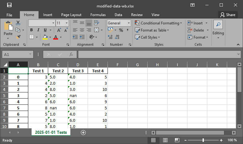
Fig. 2 The xlsx output file produced with pandas.

Note

pandas tries to convert all data into dtype=float, but as soon as there is only one text variable in a column, the entire column will be saved as string-data type in a workbook.

A pandas ExcelWriter object can be created to write multiple pd.DataFrame objects to a workbook, on one or more sheets. Here is an example, where the non-numeric "nan" strings are replaced in measurement_data with np.nan to yield a purely numeric data frame in two steps (# (1) and # (2)):

measurement_data = measurement_data.replace("nan", np.nan, regex=True)  # (1) replace "nan" with np.nan
measurement_data = measurement_data.apply(pd.to_numeric)  # (2) convert all data to numeric

# write workbook with pd ExcelWriter object
with pd.ExcelWriter("data/modified-data-wb-EW.xlsx") as writer:
    measurement_data.to_excel(writer, sheet_name="2025-01-01 Tests")
    df.to_excel(writer, sheet_name="pandas example")

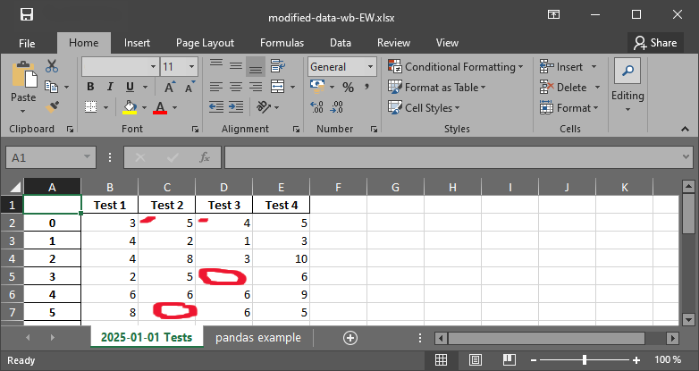
Fig. 3 The xlsx file with nan strings.

Categorical Data

string variables that represent statistically relevant categories are the baseline for data classification and statistics. pandas provides the special data type of dtype="category" to facilitate statistical analyses.

In the above Froude-number example, we used five categories to classify the flow regime as a function of the Froude number, which can serve as categories. This is useful, for instance, when no water was flowing or when a sensor broke in an experiment and we want to categorize our measurements to filter valid tests only:

flow_regimes = ["fluvial", "nearby critical (slow)", "critical", "nearby critical (fast)", "super-critical"]
observation_examples = ["fluvial", "dry", "critical", "nearby critical (slow)", "measurement error"]
Fr_cat = pd.Categorical(observation_examples, categories=flow_regimes, ordered=False)
print(pd.Series(Fr_cat))

0                   fluvial
1                       NaN
2                  critical
3    nearby critical (slow)
4                       NaN
dtype: category
Categories (5, object): ['fluvial', 'nearby critical (slow)', 'critical', 'nearby critical (fast)', 'super-critical']

Data Frame Statistics

pandas has efficient routines to perform workbook-like row or column sorting (e.g., df.sort_index() or df.sort_values()), and enables the fast calculation of data frame statistics with df.describe(), where 25%, 50%, and 75% represent the i-th percentiles:

measurement_data.describe()

	Test 1	Test 2	Test 3	Test 4
count	18.000000	16.000000	15.000000	18.000000
mean	4.111111	4.250000	4.533333	5.555556
std	2.298053	2.792848	2.386470	2.617188
min	1.000000	1.000000	1.000000	1.000000
25%	2.250000	2.000000	3.000000	4.000000
50%	4.000000	4.000000	4.000000	5.500000
75%	5.000000	6.000000	6.000000	7.000000
max	9.000000	10.000000	9.000000	10.000000

Statistical pandas data frame methods overlap with NumPy methods and include:

• df.abs() calculates asbolute values

• df.cumprod() calculates the cumulative product

• df.cumsum() calculates the cumulative sum

• df.count() counts the number of non-null observations

• df.max() calculates the maximum value

• df.mean() calculates the mean (average)

• df.min() calculates the minimum value

• df.mode() calculates the mode

• df.prod() calculates the product

• df.std() calculates tthe standard deviation

• df.sum() calculates the sum

print("Mean:\n" + str(measurement_data.mean()))
print("Median:\n" + str(measurement_data.median()))
print("Standard deviation:\n" + str(measurement_data.std()))

Mean:
Test 1    4.111111
Test 2    4.250000
Test 3    4.533333
Test 4    5.555556
dtype: float64
Median:
Test 1    4.0
Test 2    4.0
Test 3    4.0
Test 4    5.5
dtype: float64
Standard deviation:
Test 1    2.298053
Test 2    2.792848
Test 3    2.386470
Test 4    2.617188
dtype: float64

Tip

pandas has many more built-in functionalities, for example, to plot histograms or any data using the matplotlib library, and machine learning.

Apply Custom (Own) Functions to Data Frames

pandas data frames have a built-in apply(fun) method that enables applying a custom function to (parts of) a pd.DataFrame object. The following code block borrows from the feet_to_meter function from the functions chapter (download converter.py). The pandas docs provide more information about the pandas.apply method.

from fun.converter import feet_to_meter

# create data frame with random integers
df = pd.DataFrame({"Feet": np.random.randint(0, 100, size=6),
                   "Meters": np.ones(6) * np.nan})

# apply feet_to_meter to the Meters columns of the data frame
df["Meters"] = df["Feet"].apply(feet_to_meter)

print(df)

   Feets   Meters
0     59  17.9832
1     60  18.2880
2     85  25.9080
3     18   5.4864
4     20   6.0960
5      3   0.9144

Dates and Time

pandas involves methods for calculations and labeling with date and time values through pd.Timestamp, which converts date-time-like strings into timestamps or creates timestamps from keyword arguments:

print(pd.Timestamp('2025-01-01T12'))
print(pd.Timestamp(year=2025, month=1, day=1, hour=12))
print(pd.Timestamp(2025, 1, 1, 12))

2025-01-01 12:00:00
2025-01-01 12:00:00
2025-01-01 12:00:00

The expression pd.Timestamp(2025, 1, 1, 12) mimics the powerful datetime.datetime API (Application Programming Interface) of the datetime Python library, which provides sophisticated methods for handling time-dependent values. While pandas’ built-in timestamps are convenient for creating time series within pd.DataFrame objects and workbook-like tables, datetime is one of the best solutions for time-dependent calculations in Python. datetime is available by default (i.e., it must not be conda or pip-installed) and is efficiently applicable, for example, to data that were collected over several years including leap years. The datetime package comes with many attributes and methods, which are documented in detail in the Python docs.

The standard usage is:

import datetime as dt
start_date = dt.datetime(2024, 2, 25, 22, 30, 0)
end_date = dt.datetime(year=2024, month=3, day=2, hour=2, minute=15, second=30)
print("Datetime variables can be subtracted:\n" + str(end_date - start_date))
print("The result is a %s object." % type(end_date - start_date))

Datetime variables can be subtracted:
5 days, 3:45:30
The result is a <class 'datetime.timedelta'> object.

dt.timedelta objects can also be separately defined:

time_diff = dt.timedelta(days=0, seconds=0, microseconds=0, milliseconds=0, minutes=0, hours=23, weeks=0)
act_time = start_date
print("Iterate from start to end date with stepsize=time_diff:")
while act_time <= end_date:
    print(act_time.strftime("%Y-%m(%h)-%d, %H:%M:%S"))
    act_time += time_diff

Iterate from start to end date with stepsize=time_diff:
2024-02(Feb)-25, 22:30:00
2024-02(Feb)-26, 21:30:00
2024-02(Feb)-27, 20:30:00
2024-02(Feb)-28, 19:30:00
2024-02(Feb)-29, 18:30:00
2024-03(Mar)-01, 17:30:00

That is all for the introduction to data and file handling. Though there is much more to data processing than shown in this chapter and the next other chapters of this eBook will occasionally feature more tools.

Exercise

Practice pandas and its csv file handling routines, as well as basic date-time handling in the flood return period calculation exercise.

Learning Success Check-up

Take the learning success test for this Jupyter notebook.

Unfold QR Code