Contributor

This chapter was written and developed by Beatriz Negreiros

Linear Regression

In this section, we will further explore the concepts of linear ML algorithms, but now our task will focus on predicting responses in terms of continuous values, instead of discrete classes as we did in linear classification. Taking the ML application mentioned in the introduction to ML, for instance, we may now want to predict how much is the amount of a chemical substance dissolved in water, rather than just if it is dissolved or not (binary classification).

Requirements

• You are familiar with machine learning terms. We recommend reading the introduction to ML section for familiarizing with the nomenclature we use throughout the website.

• You are familiar with fundamental linear algebra concepts (such as a dot product, vector projections, planes, eigenvectors and eigenvalues). Please refer to the videos of 3Blue1Brown for a suitable revision if necessary.

• Basic knowledge in differential calculus (derivation through the chain rule, gradients).

Linear regression focuses on modeling the relationship between input variables (features) and a continuous target variable. It assumes a linear relationship between the input features and the target variable.

Note

A linear relationship is any relationship between two variables that follows a line in the coordinate space. In contrast, non-linear relationships involve non-proportionality between inputs and outputs, which may be related to thresholds, loops, or any function which does not follow the equation of a line (\(y = a \cdot x + b\)).

Here our goal is again to find the best-fitting line (or hyperplane in higher dimensions) that minimizes the difference between predicted and actual target values. To this end, we will cover:

• The least squares criterion for quantifying the training error in linear regression

• The stochastic gradient descent (SDG) algorithm, which is used in training process of a linear regression model

• The regularization term for linear regression

• The sources of error in linear regression

Empirical Risk Minimization (ERM)

Objective function

As we saw in the introduction to ML, the goal of ML is to minimize the objective function by adjusting the model’s parameters through techniques (i.e., optimization algorithms) such as gradient descent.

One of the objective functions that we may use in linear regression is Empirical Risk (\(R\)). We express the empirical risk in terms of a loss measure, which reflects only the deviation between model predictions and the target values (or labels) of our training dataset, and thus does not consider regularization. The goal of empirical risk (\(R\)) minimization (ERM) is to find a model that minimizes the discrepancy between predictions and observations on the training data, with the assumption that it will generalize well to unseen data. So we can define \(R\) as following:

\[ R(\theta) = \frac{1}{n} \sum_{t=1}^n Loss(y^{(t)}-\theta \cdot x^{(t)}) \]

where \(n\) is the number of training examples, \((x^{(t)}, y^{(t)})\) is the \(t\)-th training example (feature vector and label, respectively), and \(Loss\) is a generic loss function. Note that $\cdot§ denotes a dot product.

Important

Note also that in our definition of empirical risk (\(R\)) above, we are ignoring the bias term (\(\theta_0\)) for simplicity.

One common way to express deviations between predictions and observations on the training data is to compute the squared error, \((y^{(t)}-\theta \cdot x^{(t)})^2\), which yields the ordinary least squares (OLS) objective function:

\[ R(\theta) = \frac{1}{n} \sum_{t=1}^n (y^{(t)}-\theta \cdot x^{(t)})^2/2 \]

Note

Squaring deviations between model predictions and label values as a loss function is a common practice to solve optimization problems due to its simplicity, differentiability, and convex behaviour. If the deviations are in average large, the squared error function will strongly penalize our model.

Know more

Squaring the deviations between model predictions and label values to use as a loss function is a common practice in optimization problems for several reasons:

• Simplicity: Squaring the deviations simplifies the mathematical formulation of the loss function. It eliminates the need to consider the direction of the deviation (positive or negative) and ensures that all deviations contribute positively to the loss. Additionally, squaring preserves the nice mathematical properties required for optimization, such as being differentiable and convex.

• Emphasizing large errors: Squaring the deviations amplifies the impact of larger errors compared to smaller errors. By squaring the deviations, the loss function penalizes significant deviations more severely, which can be desirable in many applications. This emphasis on large errors can lead the optimization process to focus on reducing outliers and improving overall accuracy.

• Differentiability: Squaring the deviations makes the loss function differentiable, which is crucial for optimization algorithms that rely on gradients to update the model parameters. The ability to compute derivatives allows efficient optimization using gradient-based methods like gradient descent or stochastic gradient descent. These methods iteratively adjust the model parameters in the direction that minimizes the loss.

• Convexity: Squared loss is a convex function, meaning it has a single global minimum. Convexity simplifies the optimization process because it guarantees that the loss function has a unique solution, and optimization algorithms can converge to that solution reliably. Non-convex loss functions may have multiple local minima, which can make optimization more challenging.

Learning algorithm

Now, we will use the stochastic gradient descent (SDG) algorithm to update our model \(\theta\). Recall that we do this by adjusting the model parameters \(\theta\) with the gradient of our objective function, i.e., empirical risk, evaluated at each training example. Thus, we nudge \(\theta\) towards the direction opposite to the gradient \(\nabla_\theta R(\theta)\). Note that the function \(R\) above, defined with the squared error as loss function, is differentiable everywhere. We compute the gradient of the empirical risk, which yields:

\[ \nabla_\theta R(\theta) = -(y^{(t)}-\theta \cdot x^{(t)}) \cdot x^{(t)} \]

Thus, we can summarize our learning algorithm as:

1. Initialize \(\theta = 0\)

2. Randomly pick \(t = {1, ..., n}\)

3. Update \(\theta\), so that:

   \[\begin{split} \theta = \theta - \eta (- (y^{(t)}-\theta \cdot x^{(t)}) x^{(t)}) \\ \therefore \theta = \theta + \eta (y^{(t)}-\theta \cdot x^{(t)}) x^{(t)} \end{split}\]

   where \(\eta\) is the learning rate.

Note that this learning algorithm is very similar to the one for the case of linear classification.

Exercise 1: Difference between learning algorithms for regression and classification

There is one major difference between this learning algorithm and the one we covered for training a linear classifier. Can you spot it? Hint: Look carefully to how the update of \(\theta\) for linear regression works.

Solution

The learning algorithm for linear regression will be adjusting \(\theta\) at every step where there was some discrepancy (\(y^{(t)}-\theta \cdot x^{(t)} \neq 0\)). Thus, we are not concerned whether there is a mistake or not, which we checked with an if clause in Linear Classification, but are rather looking for how much was the discrepancy. If the prediction and the correct value deviate a lot, then the algorithm will make sure to correct \(\theta\) more strongly and, if the discrepancies are small, the algorithm will be correcting less.

Regularization: Ridge regression

Objective function

So far, our optimization problem for training a linear regression model has only focused on minimizing the training error (empirical risk minimization or ERM). However, a regularization term is crucial in most cases otherwise our model can’t generalize for other datasets (in addition to the training dataset in hands). Thus, we will now introduce a regularization term to our objective function, which now constitutes a ridge regression problem. Ridge regression introduces a regularization term, often called the “ridge penalty” or “L2 penalty” to the ordinary least squares (OLS) objective function. This penalty term (\(\frac{1}{2} \| \theta \|^2\)) controls the complexity of the model by shrinking \(\theta\) (i.e., regression coefficients) towards zero. Thus, the objective function \(J(\theta)\) for ridge regression is:

\[ J(\theta) = \frac{\lambda}{2} \| \theta \|^2 + R(\theta) \]

where \(\lambda\) is the regularization parameter we covered in the Linear Classification.

Learning algorithm

As we did in the Empirical Risk Minimization (ERM) method, we can also apply the stochastic gradient descent algorithm in ridge regression, only now we need to take the gradient of the new objective function (\(\nabla_\theta J(\theta)\)) and use it to update \(\theta\) at each iteration through the training dataset.

Let’s first expand all terms of \(J(\theta)\):

\[ J (\theta)= \frac{\lambda}{2} \| \theta \|^2 + R (\theta) = \frac{\lambda}{2} \| \theta \|^2 + \frac{1}{n} \sum_{t=1}^n \frac{(y^{(t)}- \theta \cdot x^{(t)})^2}{2} \]

The gradient can be computed now as:

\[ \nabla_\theta J(\theta) = \lambda \theta - (y^{(t)}- \theta \cdot x^{(t)}) x^{(t)} \]

Thus, we can summarize our learning algorithm as:

1. Initialize \(\theta = 0\)

2. Randomly pick \(t = {1, ..., n}\)

3. Update \(\theta\), so that:

   \[\begin{split} \theta = \theta - \eta (\lambda \theta - (y^{(t)} - \theta \cdot x^{(t)}) x^{(t)}) \\ \end{split}\]

   where \(\eta\) is the learning rate.

Exercise 2: Simplify and understand the expression of the update of \(\theta\) for ridge regression

Try to simplify the expression above that updates the value of \(\theta\) at each iteration. Hint: You will end up with a sum of two terms. What is each of these terms trying to achieve during the optimization?

Solution

Simplifying the update expression yields:

\[ \theta = (1 - \eta \lambda) \theta + \eta (y^{(t)} - \theta \cdot x^{(t)}) x^{(t)} \]

The second term of the expression, \((y^{(t)}-\theta \cdot x^{(t)}) x^{(t)}\), is exactly what we had seen before in ERM (before we added regularization). The first term, \((1-\eta \lambda)\), is trying to keep \(\theta\) as close as possible to zero, since both \(\lambda\) (regularization term) and \(\eta\) (learning rate) are positive numbers. Thus, the second term is correcting our model parameters \(\theta\) towards minimizing the training loss, whereas the first term tries to keep \(\theta\) as small as possible.

Note that by adding a regularization term to our objective function, we are now concerned with finding an optimal model that, rather than fitting the training data perfectly, it is able to generalize to other datasets as well. We do so because we believe that the model should not be adjusted to every single piece of weak evidence or noise contained in the training dataset. Instead, we introduce the regularization parameter \(\lambda\), which avoids that \(\theta\) changes except for when the evidence is strong enough to worth an increase of \(\theta\). As the value of \(\lambda\) increases, so does the training error, but with the hope that our model will generalize better, yielding a lower test error.

Structural vs. estimation error

When selecting a ML algorithm, we make certain assumptions about the relationship between the features and the labels. In the case of linear regression, the assumption is that the relationship between the features and the labels can be represented by a linear equation. If this assumption is violated, such as when the true relationship is nonlinear, then our model will have a high structural error because it cannot accurately capture the underlying patterns in the data. Thus, structural error encompasses the limitations or assumptions made by the chosen model, and it represents the irreducible error that cannot be eliminated regardless of the amount of training data. Estimation error, on the other hand, arises from the finite nature of the training data and the resulting inability of our model to fit or generalize from that data. Estimation errors can occur when the available training data is limited or does not adequately represent the true underlying distribution of the problem. In such cases, the model may struggle to capture the true patterns and relationships present in the data, leading to higher estimation errors.

Exercise 3: Sources of error in linear regression

Which of the figures below better depicts structural and estimation errors, respectively? The blue points denote the training dataset and the orange line the linear regression model.

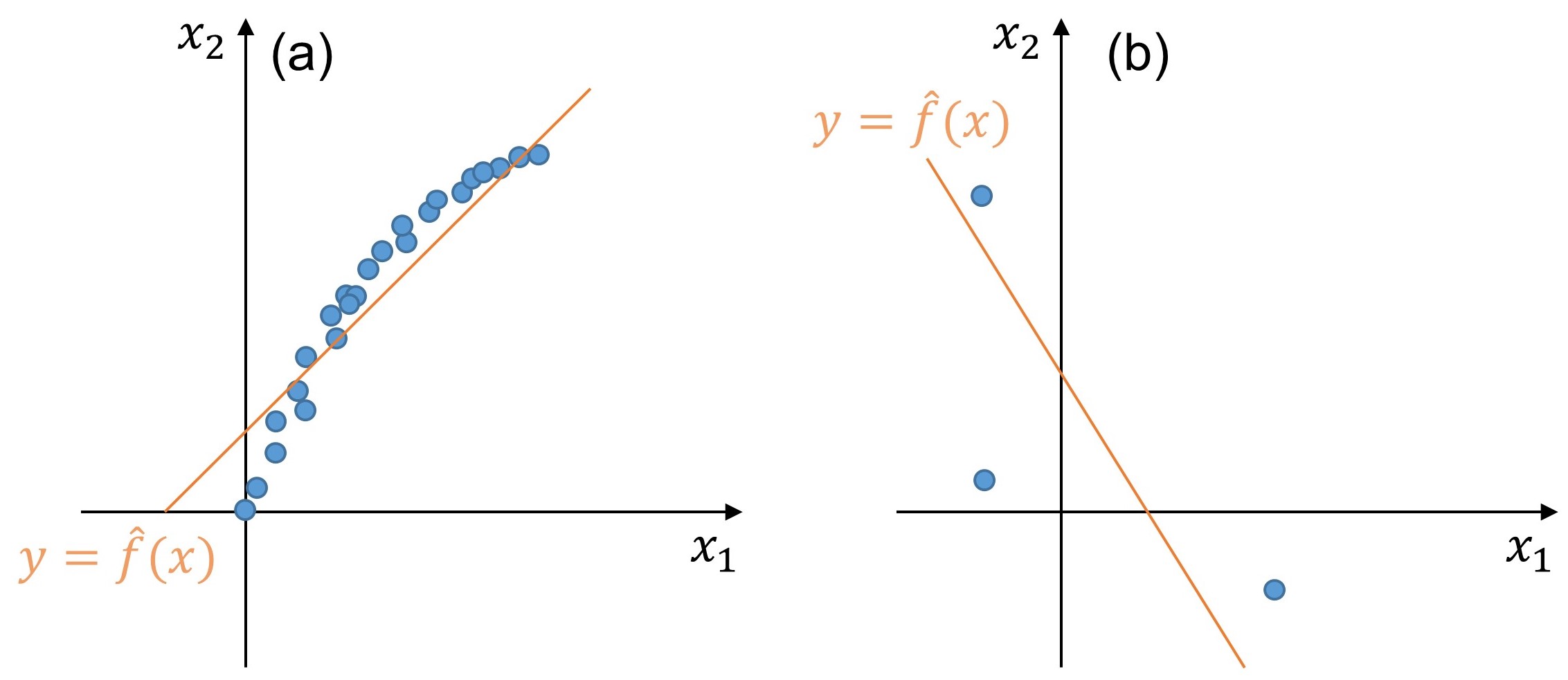
Fig. 253 Illustrative example of structural and estimation errors.

Solution

Table 16 Solution to the Machine Learning Exercise 3.

Plot	a	b
Error type	Structural	Estimation